Introduction
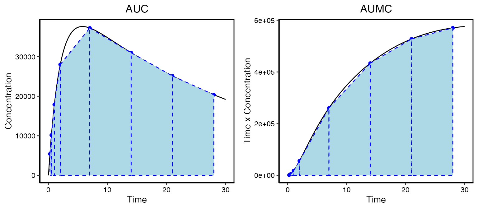
Non-compartmental analysis (NCA) is a simple and quick method for evaluating the exposure of a drug. It allows you to evaluate things like linearity and in vivo exposure. To illustrate this consider an antibody given in a subcutaneous injection. The actual profile a patient might experience is given in the solid black line. But we don’t yet have the ability to sample in a continuous fashion. What we might observer is given by the blue points.

Generally NCA will determine the following directly from the data:
-
Cmax- Maximum observed concentration (units=concentration) -
Tmax- The time where the maximum concentration was observed (units=time) -
AUC- The area under the curve (units=time \times concentration) -
AUMC- The area under the first moment curve (units=time^2 \times concentration)
These properties are all based on observational data. So the
Cmax and Tmax will most certainly not be at
the actual maximum concentration but as long as we sample judiciously it
will give us a good approximation. Similarly, the calculated
AUC and AUMC will be different than the actual
values. To calculate the areas you need to dig back into your calculus
text books to the trapezoid method. Basically each sampling interval is
a trapezoid and the area of each is calculated and added up for all of
the n samples:
AUC = \int_0^{t_f} Cdt \approx \sum_{i=1}^{n-1}{\frac{C_i+C_{i+1}}{2}\times (t_{i+1}-t_{i})} AUMC = \int_0^{t_f} t\times Cdt \approx \sum_{i=1}^{n-1}{\frac{t_iC_i+t_{i+1}C_{i+1}}{2}\times (t_{i+1}-t_{i})}
This can be done in Excel pretty easily. Depending on the data and the analysis other properties can be calculated. For example we can calculate the clearance, steady-state volume of distribution and terminal half-life:
- Clearance: CL = \frac{Dose}{AUC}
- Mean residence time: MRT = \frac{AUMC}{AUC}
- Steady state volume of distribution: V_{ss} = MRT \times CL
- Half-life: Terminal slope of the natural log of the data
Properties like AUC and AUMC can also be be calculated using extrapolation from the last time point to infinity to account for data beyond the observations at hand. The subsequent values of clearance, volumes of distribution, etc can also change with extrapolation.
There is a lot of nuance associated with these calculations, and it
is good to rely on software that focuses on this type of analysis. The
PKNCA
package has been developed with this in mind. Ubiquity provides a set of
functions to automate NCA and reporting for preclinical data. These
functions act as a wrapper for the PKNCA package which does
most of the heavy lifting. Only a small subset of the PKNCA
functionality is used here. If more extensive analysis is necessary then
PKNCA can be used directly.
This vignette contains a series of examples on how to perform NCA in ubiquity. To make a copy of these scripts and other supporting files in the current working directory run the following:
library(ubiquity)
fr = workshop_fetch(section="NCA", overwrite=TRUE)
This creates several files in the working directory. First are data sets:
-
pk_all_sd.csv- PK data for multiple subjects dosed either IV or SC at different levels -
pk_all_md.csv- Multiple dose data with intensive sampling on the first and last dose -
pk_sparse_sd.csv- Single dose data with sparse sampling
Next the following scripts demonstrate how to perform NCA:
-
analysis_nca_sd.R- Single dose data for individuals -
analysis_nca_md.R- Multiple dose data for individuals -
analysis_nca_sparse.R- Average NCA when analyzing sparsely sampled data
Quick Template for Running NCA
You should read the rest of the vignette below to understand the required data format and how the functions work. But if you are returning to this and you just want a template for running NCA you can use the following:
library(ubiquity)
cfg = build_system()
fr = system_fetch_template(cfg, template = "NCA")
This will create the file analysis_nca.R in the current
working directory. You can just uncomment/edit that script to get
started.
Single Dose Data
This example follows the script analysis_nca_sd.R, and
uses the dataset pk_all_sd.csv.
Expected Format of Data
First we build the system and load the dataset.
cfg = build_system(system_file="system.txt")
cfg = system_load_data(cfg, dsname     = "PKDATA",
                            data_file  = "pk_all_sd.csv")
The NCA functions in ubiquity expect data to have a certain format. There are columns that are required, those that are optional or depend on the kind of analysis being performed and other columns can also be present. In this context consider the following dataset:
The required columns and their names in this dataset provided in parenthesis are:
-
ID- Unique subject identifier (ID) -
TIME- Time since the first dose (TIME_HR) -
NTIME- Nominal time since the last or most recent dose (since we are dealing with single dose data this is alsoTIME_HR) -
CONC- Observed concentration for this record (C_ng_mlin ng/ml) -
DOSE- Dose given (DOSEin mg) -
ROUTE- Route of administration (ROUTE); can be either:iv bolus,iv infusionorextra-vascular
Optional columns include:
-
DOSENUM- When analyzing multiple dose data (example below), this column will be used to associate records with doses -
BACKEXTRAP- Back-extrapolation of IV data can be done generally for the entire dataset or this column can be used to specify the number of points to use on an individual basis -
SPARSEGROUP- Grouping for sparse sampling data where you want to average data at each time point
NCA and Outputs
Next we perform the NCA using system_nca_run:
cfg = system_nca_run(cfg,  dsname        = "PKDATA",
                           dscale        = 1e6,
                           analysis_name = "pk_single_dose",
                           extrap_C0     = FALSE,
                           dsmap         = list(TIME    = "TIME_HR",
                                                NTIME   = "TIME_HR",
                                                CONC    = "C_ng_ml",
                                                DOSE    = "DOSE",
                                                ROUTE   = "ROUTE",
                                                ID      = "ID"),
                           NCA_options   = list(max.aucinf.pext  = 10) )
We link the analysis to the dataset by specifying the dataset name
(dsname) used when we load the dataset. Data can be
filtered either before it’s loaded or by using the optional
dsfilter input (not used here). The dosing in the dataset
is in mg (i.e. 30 mg dose), but the mass units of the concentration
values are in ng (i.e. ng/ml). The dscale input converts
the mass units in the dose to the mass units in the observed
concentration. The analysis_name 1 is used both to refer
to this analysis in the reporting function as well as in the files
generated by the analysis. By default the initial concentration (nominal
time zero) will be back-extrapolated but can be disabled by setting
extrap_C0 to FALSE. Next we map the columns in the dataset
to names used by the analysis (dsmap). Note that both the
actual time (TIME) and nominal time (NTIME)
both use the same column in the dataset (TIME_HR). Lastly,
the NCA_options can be used to specify the analysis options
used by PKNCA. In the example above the maximum percent of AUCinf
extrapolation is being specified at 10%. This will only change this
option and the remaining defaults from PKCNA will be used. Either omit
this argument or set it to NULL to use all of the PKNCA defaults.
Running this function will produce the following files:
-
output/pk_single_dose-nca_summary-pknca.csvSummary level output from the analysis (see table below) -
output/pk_single_dose-nca_data.RDataR objects used for downstream reporting -
output/pk_single_dose-pknca_raw.csvRaw output from PKNCA
It may be useful to carry forward the values of certain columns in
the PK dataset into the output. To do this you can use the
dsinc argument and provide a list of columns in your input
dataset to be appended to the summary table. You can access the summary
table using the function system_fetch_nca and the
analysis_name:
NCA_results = system_fetch_nca(cfg, analysis_name = "pk_single_dose")To get an explanation of the columns in the NCA output you can use
the system_fetch_nca_columns function passing the NCA
analysis name to the function. The list output contains a data frame
NCA_col_summary with the outputs and a description of their
meaning:
nca_cols = system_fetch_nca_columns(cfg, "pk_single_dose")
rhandsontable(nca_cols[["NCA_col_summary"]],  width="100%", height=200)
Automated Reporting
PowerPoint
Once the NCA has been run, the results can be appended to an open
PowerPoint report. Here we initialize an empty report then use the
function system_rpt_nca() and the analysis name assigned to
the analysis above (pk_single_dose) to attach those
results. Then we can write the file:
cfg = system_rpt_read_template(cfg, template="PowerPoint")
cfg = system_rpt_add_slide(cfg,
  template = "title_slide",
  elements = list( title= list(content = "NCA Single Dose PK", type    = "text")))
cfg = system_rpt_nca(cfg=cfg, analysis_name="pk_single_dose")
system_rpt_save_report(cfg=cfg, output_file=file.path("output","pk_single_dose-report.pptx"))
For each dose a summary slide will be produced and a full timecourse will be created showing all of the data for that subject/group in the dataset:
- Actual data in gray
- Data used for NCA in green
- Initial extrapolated concentrations in orange (solid)
- Points used for extrapolating “iv bolus” data are shown in orange open circles
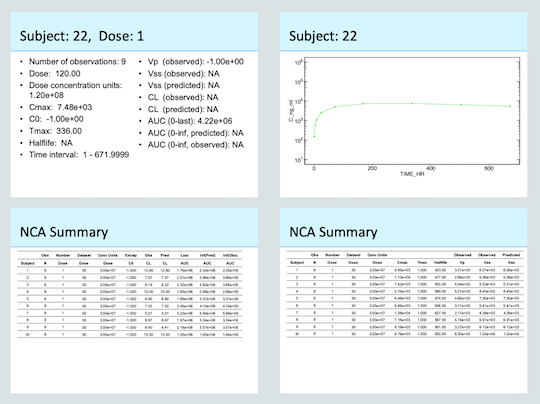
Below shows the slides generated for an individual subject and the
first set of summary slides for the analysis. Notice that because
extrap_C0 was set to FALSE C0 was not
calculated (-1). Because this individual received a SC dose
the estimate for Vp is also not calculated
(-1). Also note that the data for this individual did not
allow for extrapolation of AUC to infinity (NA). As a
result the parameters that depend this value also resulted in
(NA). The timecourse figure shows the data in the dataset
(gray closed symbols, solid line) and the data used for NCA (green open
symbols, dashed line). This way you can visually confirm at the subject
level what data was used.

Word
Similarly, a Word report can be generated by appending the results to
an already initialized Word report. This is done by setting the
template to "Word" when calling
system_rpt_read_template(). This will attach the same
content to the report as with PowerPoint report above.
cfg = system_rpt_read_template(cfg, template="Word")
cfg = system_rpt_nca(cfg=cfg, analysis_name="pk_single_dose")
system_rpt_save_report(cfg=cfg, output_file=file.path("output","pk_single_dose-report.docx"))
For more information on integrated report generation see the
Reporting vignette.
Summarizing Data
The automated reporting is intended to generate results quickly in an
easily digestible way (Word and PowerPoint). But you may decided you
need more control over what is being presented. The function
system_fetch_nca() mentioned above will give you access to
all of the NCA output. If you want to filter, select columns and
summarize results the function system_nca_summary() can be
used. The first argument (analysis_name) indicates the NCA
analysis you want to summarize. The parameters being summarized and
their order in the table is specified by params_include. By
default internal headers will be used, but you can overwrite or alter
those defaults with optional params_header input. Here
cmax is being overwritten with the internally predefined
label ("<label>") on the first header row, and the
units ("(ng/ml)") on the second header row. In this table
we only want to present the 30 mg dose. The ds_wrangle
option will filter down the results to just that dosing cohort. It may
be desirable to further summarize results. The
summary_stats option is a list of values to summarize and
the columns where those summaries should appear. Each name in that list
will create a row at the bottom of the column. You can specify the
summary labels with summary_labels and indicate which
column to contain those labels with summary_location.
nca_table = system_nca_summary(cfg,
       analysis_name    = "pk_single_dose",
       params_include   = c( "ID", "cmax", "tmax", "half.life", "auclast"),
       params_header    = list(cmax = c( "<label>", "(ng/ml)")),
       ds_wrangle       = "NCA_sum = NCA_sum %>% dplyr::filter(Dose == 30)",
       summary_stats    = list("<MEAN> (<STD>)" = c("auclast", "half.life"),
                               "<MEDIAN>"       = c("tmax")),
       summary_labels   = list(MEAN             = "Mean",
                               STD              = "Std Dev",
                               N                = "N obs",
                               MEDIAN           = "Median",
                               SE               = "Std Err."),
       summary_location = "ID")

nca_table[["vignette"]] = set_table_properties(nca_table$nca_summary_ft,layout = "autofit")
The output of system_nca_summary() is a list with
elements that are designed to facilitate reporting. The unformatted
tabular information is provided in a dataframe
(nca_summary) and this can be saved as text for archival
purposes. Flextable output (nca_summary_ft) is also
provided. This can be further customized if needed and eventually be
used in Word or PowerPoint (see below). If you want to create your own
output from this you can use the components field.
ID |
Cmax |
Tmax |
Half-life |
AUC last |
|---|---|---|---|---|
(ng/ml) |
||||
1 |
9,950 |
1 |
423 |
1,760,000 |
2 |
11,300 |
1 |
477 |
2,510,000 |
3 |
7,420 |
1 |
500 |
2,320,000 |
4 |
5,760 |
1 |
589 |
1,650,000 |
5 |
6,460 |
1 |
574 |
1,890,000 |
6 |
9,460 |
1 |
526 |
2,450,000 |
7 |
13,800 |
1 |
627 |
3,230,000 |
8 |
7,160 |
1 |
567 |
1,970,000 |
9 |
9,180 |
1 |
561 |
2,180,000 |
10 |
4,760 |
1 |
500 |
1,250,000 |
11 |
4,670 |
1 |
599 |
1,630,000 |
12 |
12,100 |
1 |
546 |
2,620,000 |
13 |
6,380 |
1 |
581 |
2,010,000 |
14 |
5,130 |
1 |
549 |
1,620,000 |
15 |
4,910 |
1 |
751 |
1,890,000 |
16 |
7,580 |
1 |
619 |
1,640,000 |
17 |
10,200 |
1 |
507 |
2,500,000 |
18 |
10,600 |
1 |
639 |
2,900,000 |
Mean (Std Dev) |
563 (73.1) |
2110000 (517000) |
||
Median |
1 |
Multiple Dose Data
This example follows the script analysis_nca_md.R, and
uses the dataset pk_all_md.csv. If we rebuild the system
and load the multiple dose dataset we can see that the dataset looks
almost identical to the single dose data set. The primary difference is
that there are two extra columns: NTIME_HR and
EXTRAP. The first column (NTIME_HR) contains
the time since the last dose. The EXTRAP column is optional
and allows the user to specify the number of points to back extrapolate
C0 for iv bolus dosing. This will have no effect unless it
is specified in the dsmap below. If you scroll through the
data you can see that there is intensive sampling for
DOSENUM 1 and 6. But for doses 2-5 there are only three
samples per interval. These latter dose intervals (2-5) will be ignored
with the default value of NCA_min (4) which defines the
minimum number of samples required for analysis.
cfg = build_system(system_file="system.txt")
cfg = system_load_data(cfg, dsname     = "PKDATA",
                            data_file  = "pk_all_md.csv")
Next we perform the NCA and reporting as before. The only difference
here is that we’ve removed the extrap_C0 option. The
default value is TRUE so back-extrapolation will occur. For
IV dosing this is log-linear extrapolation to a nominal time of zero.
For SC dosing this will be 0 for the first dose and the last observation
from the last dosing interval for subsequent dosing.
cfg = system_nca_run(cfg, dsname        = "PKDATA",
                          dscale        = 1e6,
                          analysis_name = "pk_multiple_dose",
                          dsmap         = list(TIME    = "TIME_HR",
                                               NTIME   = "NTIME_HR",
                                               CONC    = "C_ng_ml",
                                               DOSE    = "DOSE",
                                               ROUTE   = "ROUTE",
                                               ID      = "ID",
                                               DOSENUM = "DOSENUM",
                                               EXTRAP  = "EXTRAP"))
cfg = system_rpt_read_template(cfg, template="PowerPoint")
cfg = system_rpt_nca(cfg=cfg, analysis_name="pk_multiple_dose")
system_rpt_save_report(cfg=cfg, output_file=file.path("output","pk_multiple_dose-report.pptx"))
The same files are generated with the pk_multiple_dose
prefix in the out output folder. The summary can be seen
here:
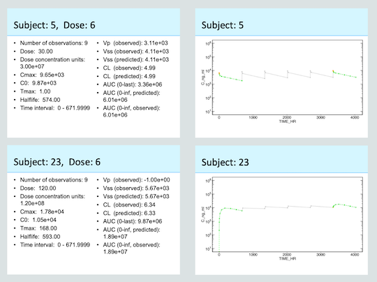
Below you can see the report slides for two subjects. The first subject was dosed IV. Again the gray markers/solid line show the full timecourse for that subject from the dataset. The data used for NCA (dose 1 and 6) is shown in green. The solid orange marker shows the extrapolated C0. If you look closely the open orange markers show the data points used for extrapolation connected with an orange dashed line. The second subject was given SC doses. For the first dose the extrapolated C0 was zero. This can be seen by the green dashed line extending down to zero. The C0 for dose 6 is simply the last observation carried forward as shown by the solid orange marker.

Sparse Sampling
This example follows the script analysis_nca_sparse.R,
and uses the dataset pk_all_sparse.csv. First we rebuild
the system and load the sparsely sampled dataset. This data is very
similar to the single dose dataset above except each ID only has three
samples.
cfg = build_system(system_file="system.txt")
cfg = system_load_data(cfg, dsname     = "PKDATA",
                            data_file  = "pk_sparse_sd.csv")
When we run the NCA we need to tell the function that we want to
perform a sparse analysis. This is done by setting the
sparse input to TRUE. We also need to provide
information on how to group cohorts. This is done by providing a
SPARSEGROUP option in the dsmap. In this case
we can just use the DOSE column, however a different column
could have been used.
cfg = system_nca_run(cfg, dsname        = "PKDATA",
                          dscale        = 1e6,
                          analysis_name = "pk_sparse",
                          sparse        = TRUE,
                          dsmap         = list(TIME        = "TIME_HR",
                                               NTIME       = "TIME_HR",
                                               CONC        = "C_ng_ml",
                                               DOSE        = "DOSE",
                                               ROUTE       = "ROUTE",
                                               ID          = "ID",
                                               SPARSEGROUP = "DOSE"))
cfg = system_rpt_read_template(cfg, template="PowerPoint")
cfg = system_rpt_add_slide(cfg,
  template = "title_slide",
  elements = list( title= list(content = "NCA of Sparsely Sampled PK", type    = "text")))
cfg = system_rpt_nca(cfg=cfg, analysis_name="pk_sparse")
system_rpt_save_report(cfg=cfg, output_file=file.path("output","pk_sparse-report.pptx"))
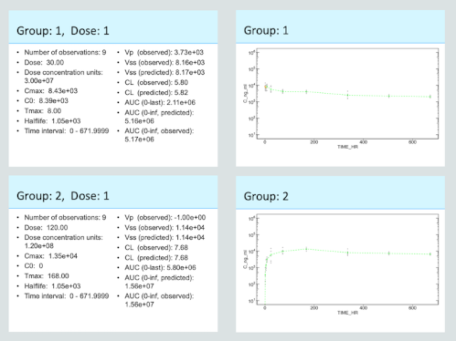
Analysis of sparse data will calculate an average concentration at each time point and use those average values for NCA. The same files are generated from the analysis. You can see the summary here:
To confirm what was done and identify any outliers that may be causing problems, you can use the report output. Again the gray markers show the data, the green dashed line will show the value used for NCA, and the orange will show the C0 estimate.

