Model Deployment

Introduction

Once a model has been developed it may be useful to provide an easy way to run simulations or automate specific analyses. Do to that, a ubiquity provides a ShinyApp that allows the model to be run from an easy to use interface that is highly customizable. This App can be run locally (useful during meetings to answer quick questions) or deployed on a Shiny server to allow others access to the model.

To demonstrate this interface we can begin with the PK model of mAbs in humans (Davda etal. mAbs, 6(4), 1094-1102) :

library(ubiquity)
system_new(file_name = "system.txt", system_file = "mab_pk", overwrite = TRUE)
cfg = build_system(system_file = "system.txt")

Use ?system_new to see a list of the available system file examples. After building any system you can then create the ShinyApp template:

system_fetch_template(cfg, template = "ShinyApp", overwrite = TRUE)

This should create the following three files:

ubiquity_app.R - Script to run and control ubiquity ShinyApp
server.R - Server script
ui.R- UI script

Running the model

Next simply open ubiquity_app.R in RStudio and source it, and RStudio will open in a window associated with that application. The ShinyApp tends to work better when run within a browser.

After starting the App will load the default dosing from the file and run the model. The first model output will be plotted. And as you make changes to the App, those changes will be reflected in the user log at the bottom of the screen. You can change the outputs being plotted, the axis limits, and other aspects of the plot using the plot controls below the figure.

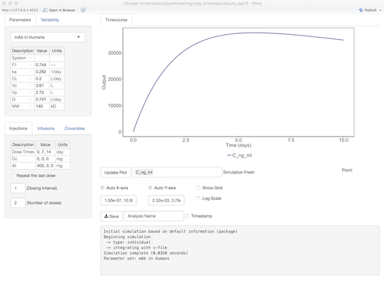
ShinyApp interface after initialization

The intent is to provide a quick method to get the model up and running with default behaviors that will provide for most of what users will need. The behavior of the ShinyApp can be further customized (described below). First we will discuss the default interface:

Altering dosing

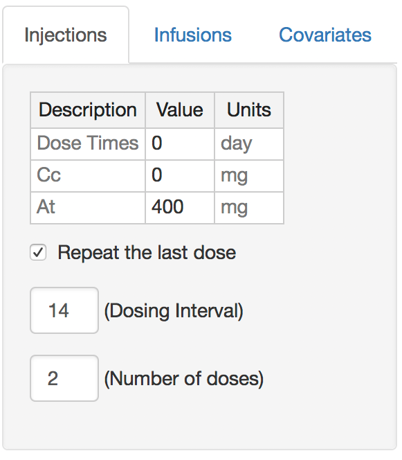
A list of bolus times and values can be specified as comma-separated values. To dose in a repeated fashion check the ``Repeat the last dose’’ box, provide a dosing interval (in the same units as the dosing times), and give the number of doses to administer. The example here will repeat the 400 mg dose every two weeks for two doses.

Bolus Dosing

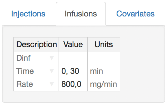
Rates of infusion are specified as a set of switching times and corresponding infusion rates (both separated by commas). The infusion rates are held constant until the next switching time. The example here would infuse the drug at 800mg/min starting at time 0, and the infusion will be turned off (set to 0) after 30 minutes.

Continuous Infusion

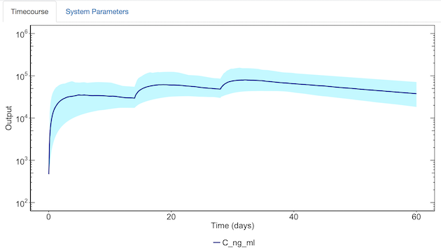
Population simulations

If the variability for system parameters has been specified (<IIV:?>? and <IIVCOR:?>?) then a “Variability” tab will be visible. Simply check the “Simulate with variability” box, alter the number of subjects, prediction interval, and elements of the variance-covariance matrix to simulate the desired population response.

Population simulation options

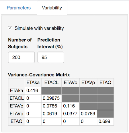
When you select “Update Plot”, each selected output will be plotted (mean – solid line, selected confidence interval – shaded region).

Population timecourse

Saving model results

Saving an analysis

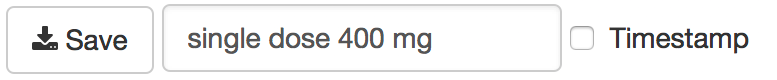
To save the model results you need to only provide a descriptive name for the analysis, push the save button, and click on the link that is generated. If you select the time stamp, this will be appended to the name of the zip file. By default the following files will be saved:

analysis_single_dose_400_mg_lib.r, analysis_single_dose_400_mg.r - These two files can be used to recreate the results from the ShinyApp.
analysis_single_dose_400_mg_timecourse.png - Time-course with the simulation results
analysis_single_dose_400_mg.csv - Predictions containing each timescale in the model, every state, and output
analysis_single_dose_400_mg_RX.html - A file for each report (X) that has been specified in ubiquity_app.R (See below)
system.txt - The system file describing the model
ubiquity_log.txt - The log file of what the user has done

Model scripts

The files analysis_NAME.r and analysis_NAME_lib.r can be used in two ways. First, these two files can be used as stand-alone files to recreate the simulation results from the ShinyApp. Creating Simulation Scripts The main script (analysis_NAME.r) can be used as a starting point to create simulation scripts. To do this it is necessary to modify First comment out the sourcing of the standalone library:

#source("analysis_NAME_lib.r");

Next (with this script and the system.txt file) uncommenting the following lines that will force the system to be rebuilt and any changes to the system file loaded.

if(!require(ubiquity)){
  source(file.path('library', 'r_general', 'ubiquity.R')) }
cfg = build_system(system_file="system.txt")

Controlling what is saved

In certain instances you may not want to allow the user access to everything that is saved by default. If you edit the ubiquity_app.R you can alter what is being pushed to the user by setting the relevant fields to FALSE.

cfg$gui$save$system_txt = TRUE
cfg$gui$save$user_log   = TRUE

Model documentation

Model diagram

It can be difficult for a user to look at a set of parameters, dosing inputs, and outputs and determine how a model works. To aid the user it can be useful to create a model diagram. To utilize the majority of the screen space, the image should be roughly twice as wide as it is tall.

You can create this image in your favorite drawing program. Inkscape is a free vector drawing program available at inkscape.org. If you run the following:

system_fetch_template(cfg, template="Model Diagram")

it will create the file system.svg. You can edit it and save it as a portable network graphics (png) file named system.png in the directory with the ubiquity_app.R file. When you start the ShinyApp it should find that file and create a tab in the plotting area of the App.

Model reports

Sometimes you need more detail than an annotated model diagram. Or you may need to perform some calculations based on the results of a simulation. It may be better to present information in a tabulated format. For these scenarios you can create an RMarkdown file. Create a copy the report template (system_report.Rmd) and a script to test it (test_system_report.r):

system_fetch_template(cfg, template="Shiny Rmd Report")

When this is called you’ll have access to the ubiquity model object (cfg) and the simulation results som. The simulation results will take the form of a deterministic simulation (see the output of ?run_simulation_ubiquity) or, if variability is checked, a stochastic simulation (see output of ?simulate_subjects)

To tell the ShinyApp to load the report (named system_report.Rmd), the following lines need to be added to ubiquity_app.R.

cfg$gui$modelreport_files$R1$title = "Tab Title"
cfg$gui$modelreport_files$R1$file  = "system_report.Rmd"

The title field is the title of the tab in the ShinyApp and file is the name of the file that you created. You can create up to five reports this way, and these are differentiated by the list name (R1, R2, … R5).

The file test_system_report.r can be used to debug your model report file. First run your model in the ShinyApp with the reports disabled. When the App runs it stores the state (cfg) and the current simulation results (som) in the following data files:

cfg \rightarrow transient/rgui/default/gui_state.RData
som \rightarrow transient/rgui/default/gui_som.RData

Next load the test script, modify the report name accordingly, and run it:

load("transient/rgui/default/gui_som.RData")
load("transient/rgui/default/gui_state.RData")
params = list()
params$cfg = cfg
params$som = som
rmarkdown::render("system_report.Rmd",
                   params = params,
                   output_format = "html_document")

This should generate your report in HTML format. You can insert debugging commands in the report and test it while you add information. Once you have it working, you can enable the report as described above and it should appear as a tab viewable by the user.

Not all reports may depend on user input. For example, if you have an RMarkdown file that documents your modeling assumptions or the model construction process then the content will not change as the user interacts with the App. To use a pre-rendered report you simply have to replace .Rmd with .html:

cfg$gui$modelreport_files$R1$title = "Tab Title"
cfg$gui$modelreport_files$R1$file  = "system_report.html"

This will tell the App to read in the html, prevent rendering the report, and speed things up for the user.

User definable functions

To customize the simulation and plotting within the ShinyApp it is necessary to create custom functions. These need to be placed in a file. For example these could be placed in mylibs.r in the main template directory. Lastly, you need to tell the ShinyApp to load this file. You need to edit ubiquity_app.R and add the following line:

cfg$gui$functions$user_def = 'mylibs.r'

Custom simulation commands

By default the ShinyApp will run simulations using run_simulation_ubiquity (individual) or simulate_subjects (population). These take as inputs the parameters vector containing the current parameter set with any changes made through the interface and cfg data structure. You can create your own functions and overwrite these by defining the following:

Individual Simulations

cfg$gui$functions$sim_ind = 'function_name(parameters, cfg)'

Population Simulations

cfg$gui$functions$sim_var = 'function_name(parameters, cfg)'

Note that in order to use the default plotting functionality these functions need to return values in the same format as the default functions for individual (run_simulation_ubiquity) and population (simulate_subjects) simulations.

Custom plotting commands

To customize the plotting output you need to create functions that can utilize the simulation output som. For individual and population simulations this is the output of run_simulation_ubiquity and simulate_subjects, respectively. Unless user-specified simulation functions are being used. In that case som can have any format needed. It is possible to also access the parameters vector containing current parameter set with any changes made through the interface and cfg data structure. You can create your own plotting functions and overwrite these by defining the following in ubiquity_app.R:

Indiviudal Plot

cfg$gui$functions$plot_ind =  'function_name(cfg, parameters,som)'

Population Plot

cfg$gui$functions$plot_var =  'function_name(cfg, parameters,som)'

Deployment on a Shiny Server

To deploy the ShinyApp on a shiny server you need to indicate this by modifying ubiquity_app.R and changing the deploying variable to TRUE:

deploying = TRUE

Then the ShinyApp needs to be initialized on the server. You can do this two ways. First you can create an empty file called REBUILD that needs to be deployed along side the other app files. You can do this with the touch command from the nat.utils package:

nat.utils::touch("REBUILD")

This will force the initialization the first time the app is loaded. This works well if you are using rsconnect to deploy your app. Alternatively, you can manually sync the files and run the following as the shiny user on the server.

R -e "source('ubiquity_app.R')"

If the App fails to run on the Shiny Server check the following:

Make sure all of the correct packages have been installed and are available to the user the Shiny Server is running under.
Make sure the ownership and permissions on the server files is correct.

To test deployment you can install the shinyVM

John Harrold & Anson K Abraham

2024-10-25